Google Sheets Basics
On that page you can find all Job Aids for each module. Click on a button to open Job Aid in a different window.
Module 1: Speeding Up Data Entry
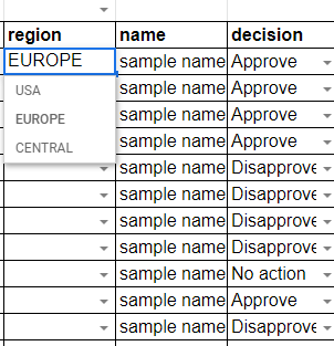
Dropdown List with Data Validation
- Choose a cell
- Click Data in the top menu
- Choose Data validation in dropdown menu
- Next to Criteria choose list of items
- Enter your items, separated by comma
- Click save
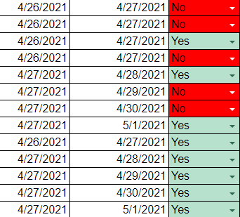
Conditional Formatting
- Choose a cell
- Choose Format in the top menu
- Create Format rules
- Choose color of your choice to your rule
- Add so many rules as your like
- Click save
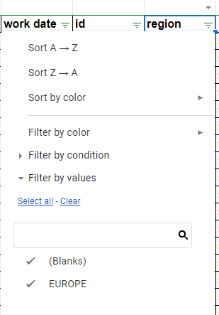
Filter View
- Choose a row or a cell
- Click Data in the top menu
- Choose Filter Views in dropdown menu
- Choose Create new filter view
- Name your filter
Module 2: Removing Duplicates Job Aid
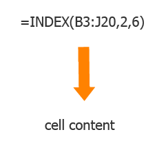
Index Function
Syntax: =INDEX(reference, row number, column number)
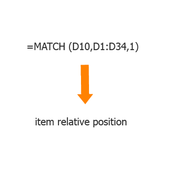
Match Function
Syntax: =MATCH (search_key, range, [search_type])
search_key - The value to search for.
range - The one-dimensional array to be searched.
search_type - [ OPTIONAL - 1 by default ] - The manner in which to search.
1, the default, causes MATCH to assume that the range is sorted in ascending order and return the largest value less than or equal to search_key.
0 indicates exact match, and is required in situations where range is not sorted.
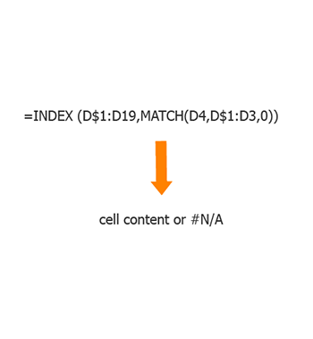
Index Match
Index Match returns the content of the cell specified by Match function. If the content is not present in the range you will see output #N/A.
=INDEX(reference, MATCH(search_key, range, search_type)).
reference - column that we want to check for duplicates. For example, D1:D20
search_key - the first cell in the column, for example, D4, later formula will be applied to the whole column
range - column before cell that contains our search key. In that case before cell D4
search_type - 0 (because we want an exact match)
$ - static indicator. When we will apply the formula all numbers that don’t have static indicator will be changed.
Module 3: Counting Data Job Aid
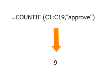
Countif Function
Syntax: =COUNTIF(range,criterion)
range - The range which is tested against criterion.
criterion - The pattern or test to apply to a range
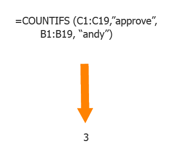
Countifs Function
=COUNTIFS(criteria_range1, criterion1, [criteria_range2, criterion2, ...])
criteria_range1 - and criterion1 - first set of range and criterion
criteria_range2 and criterion2, - second set of range and criterion
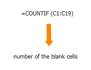
Countblank Function
The Countblank function returns the number of the black cells across given range =COUNTBLANK(range).
range - The range where you want to find blank cells.
Next ⇨